Assume that a procedure yields a binomial distribution. This assumption underlies many statistical analyses and provides a powerful tool for modeling phenomena with binary outcomes. Understanding the assumptions and properties of the binomial distribution is essential for accurate interpretation and application.
In this comprehensive guide, we will explore the concept of the binomial distribution, its probability mass function, mean and variance, and practical applications. We will also discuss extensions and generalizations of the binomial distribution, providing a thorough understanding of this fundamental statistical concept.
Binomial Distribution: Assume That A Procedure Yields A Binomial Distribution

A binomial distribution models the number of successes in a sequence of independent experiments, each of which has a constant probability of success.
The binomial distribution is often used to model phenomena such as the number of heads obtained when flipping a coin, the number of defective items in a batch of products, or the number of customers who visit a store on a given day.
Assumptions
- The number of experiments, n, is fixed.
- The probability of success, p, is the same for each experiment.
- The experiments are independent.
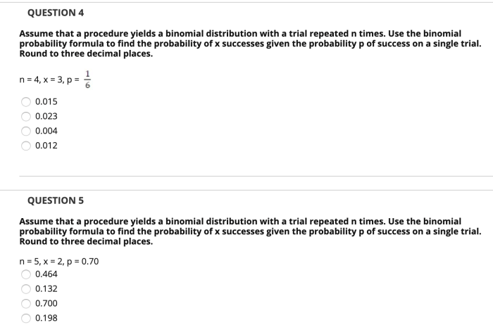
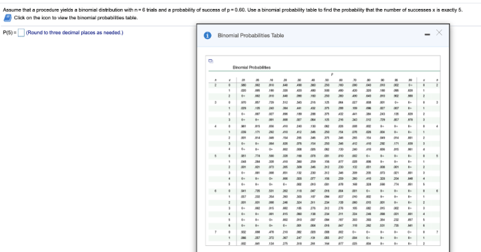
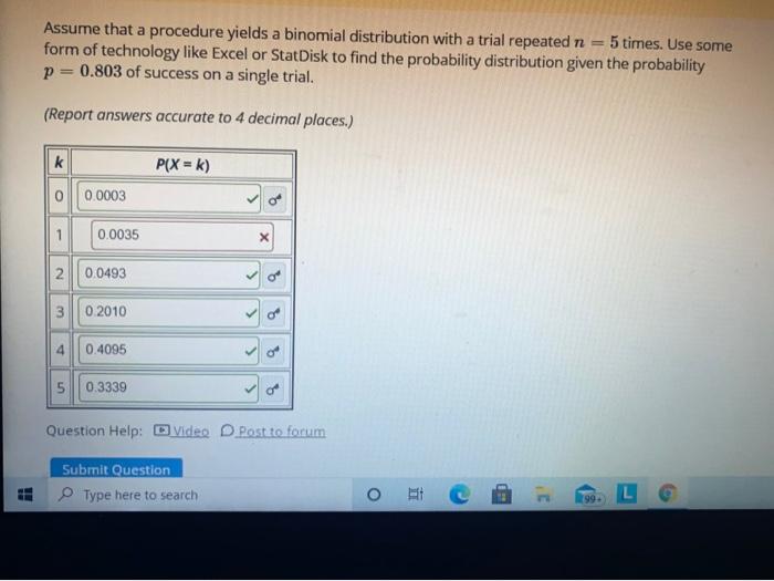
Probability Mass Function
The probability mass function of a binomial distribution is given by:
P(X = k) = (n choose k)
- p^k
- (1
- p)^(n
- k)
where:
- X is the number of successes
- n is the number of experiments
- p is the probability of success
- (n choose k) is the binomial coefficient, which represents the number of ways to choose k successes from n experiments
Mean and Variance
The mean of a binomial distribution is given by:
μ = n
p
The variance of a binomial distribution is given by:
σ^2 = n
- p
- (1
- p)
Examples and Applications, Assume that a procedure yields a binomial distribution
Binomial distributions are used in a wide variety of applications, including:
- Quality control: To model the number of defective items in a batch of products
- Marketing: To model the number of customers who visit a store on a given day
- Epidemiology: To model the number of people who contract a disease
Extensions and Generalizations
There are a number of extensions and generalizations of the binomial distribution, including:
- Negative binomial distribution: Models the number of failures until a specified number of successes
- Beta-binomial distribution: Models the probability of success in a sequence of experiments where the probability of success varies from experiment to experiment
FAQ Insights
What are the key assumptions of the binomial distribution?
The binomial distribution assumes that each trial has only two possible outcomes, the probability of success remains constant throughout the trials, the trials are independent, and the number of trials is fixed.
How is the probability mass function of the binomial distribution calculated?
The probability mass function of the binomial distribution is given by: P(X = x) = (n! / (x!(n-x)!)) – p^x – (1-p)^(n-x), where n is the number of trials, x is the number of successes, and p is the probability of success.